The News Inflationary Pressures Indices are our diffusion index summarizing inflation news. We put them through thorough testing to check whether they formally lead overall inflation data in the US and the euro area. The procedure and results are extensively discussed in this note and they bring evidence that the NIPI can be considered a leading indicator, with up to 3 months lead over official inflation releases.
The one, obvious, but tricky, question that comes most often in presentations:
- How do you know your models and data "work"?
By that, one means: what is the statistical evidence that the data can help forecast inflation, for instance?
Of course, our language models have been thoroughly tested. We know they are able to detect news potentially relevant to near-term inflation, through historical test sets analysis on labeled data, as well as out-of-sample observations throughout the COVID and post-COVID periods.
But that falls short of traditional time-series analysis. To the question on quantitative and systematic evidence about a lead-lag relationship, the honest answer until now has been: we just cannot reliably measure those effects at this point.
The limiting factor has been the data sample length, with our data starting the 1st of January 2018. When the models were designed, there was a trade-off between compehensiveness and historical record length. We chose comprehensiveness (and timeliness). The NewsBots and NIPI databases rely on hundreds of thousands of news websites queried every day. It is only a question of time, with live models and data, before we get both comprehensiveness AND historical records...
Now, the good news is: we are getting there.
We now have almost 80 monthly data points, an acceptable starting point for regular time-series analysis (our data has a daily frequency, but if we want to compare with, say, CPI, the frequency will be reduced to monthly).
Besides, with the current inflation slowdown post-COVID, we are now getting a step closer to a full inflation cycle in our sample, with high and low phases, or at least both upside and downside surprises.
It now makes sense to provide time-series statistical evidence to this critical question: do the NIPI time series, which summarize and quantify all the inflation information we gather, actually lead official inflation data?
The purpose of this note is to present a first batch of those evidence. We will explain in great detail the data under review and the framework to respond the lead-lag question. Readers mostly interested in the results can jump to the final parts. And here's a teaser, too: yes, the NIPI data lead inflation over the next 2-3 months and, in several key aspects, the results actually exceed our own expectations.
Data under review
Our benchmark short-term inflation momentum metrics will be month-on-month seasonally adjusted (SA) inflation rates. Despite their critical importance, reliable SA inflation indices are relatively rare (for reasons beyond the topic discussed here), so we will stick with a couple of well-established benchmarks in this analysis.
In the United States, the Bureau of Labor Statistics (BLS) provides seasonally adjusted Consumer Price Indices (CPI), which serve as a primary reference. Similarly, in the Euro area, the European Central Bank (ECB) produces a seasonally adjusted Harmonized Index of Consumer Prices (HICP) series, based on Eurostat data. The ECB indices occasionally experience residual disturbances from working-day or calendar-related effects, more so than the US BLS CPI data, but they are, for the most part, rather reliable.
Our analysis includes both headline CPI-HICP and CPI-HICP excluding food and energy (Core inflation). Additionally, we incorporate a couple of "supercore" measures, in order to explore whether the News Inflationary Pressures Indices (NIPI) can provide leading signals for these metrics, too. In theory, the NIPIs most likely should NOT lead those. They have been designed to capture hard-to-forecast, idiosyncratic, short-term shocks. In the long-term, those shocks are expected to cancel out and the NIPIs should be "converging" towards the supercore "trend" measure. But the long term can be a particularly remote prospect.
We also include some other key sub-indices, such as core goods and services (core services in the US, overall services in the euro area) and we will compare those to the core NIPIs.
One key consideration to the lead-lag analysis is data release frequency and timing alignment:
- the NIPI has a daily frequency and is available next day (t+1);
- the official inflation data frequency is monthly and the data are released either at the end of the month (EA HICP) or around the middle of the following month (US CPI).
To avoid any look-ahead bias, it is necessary to adjust the dates of the HICP and CPI indices forward to reflect their actual release dates. This ensures that the analysis is conducted in a manner consistent with how data would be available in real-time.
The cut-off date to our database is the first of August 2024. The last data points used in our database are therefore the US CPI June 2024 release (effective release date: 11th of July), HICP July 2024 (effective release date: 31st of July) and the 31st of July NIPI data point (released the next day).
Table 1 details the source series codes for each inflation time series and the respective adjustments applied ("shift", in days). We utilize here pseudo real-time data: the proxy rule closely approximates real release times, typically deviating from actual dates by only a few days.
| Region | Name | Source | Source code | Macrobond code | Shift (days) |
|---|---|---|---|---|---|
| US | Headline CPI | BLS | CUSR0000SA0 | uspric2156 | 44 |
| Core CPI | BLS | CUSR0000SA0L1E | uspric2373 | 44 | |
| Trimmed mean 3m PCE | FRB Dallas | rel_usdalfedtrimpce | uspric0049 | 58 | |
| Core Goods CPI | BEA | cusr0000sacl1e | bls_cusr0000sacl1e | 44 | |
| Core Services CPI | BEA | cusr0000sasle | bls_cusr0000sasle | 44 | |
| Euro area | Headline HICP | ECB | ICP.M.U2.Y.000000.3.INX | ecb_00678029 | 30 |
| Core HICP | ECB | ICP.M.U2.Y.XEF000.3.INX | ecb_00678040 | 30 | |
| Supercore HICP | ECB | ICP.M.U2.N.SPRXEF.3.INX | ecb_00993631 | 45 | |
| Core Goods HICP | ECB | ICP.M.U2.Y.IGXE00.3.INX | ecb_00678036 | 30 | |
| Services HICP | ECB | ICP.M.U2.Y.SERV00.3.INX | ecb_00678037 | 30 |
Most critically, the exercise is overly demanding on the NIPI because it does not really leverage on the NIPI's daily frequency. We are only looking at the information set at the CPI release proxied date, and then at exactly 1 month, 2 months intervals etc, day for day, before the release date. We do not incorporate any NIPI information available in between these monthly points. Whatever the outcome, it is reasonable to expect the results could be further improved by optimizing the NIPI reference days.
Granger-causality framework and implementation
To determine whether one time series leads another, the standard statistical test is Granger causality.
The framework is linear, so it will not cover steps or threshold effects (for instance turning points) which are non-linear; but it is still a well-rounded starting point to our analysis.
The Granger causality test examines whether the inclusion of past values of variable x enhances the forecasting accuracy of variable y. If x past values provide significant predictive power for y current values, then we conclude that x Granger-causes y.
Despite the name, the test evaluates lead-lag relationships, not actual "causality".
In our context, the test implementation involves three steps:
1. Stationarity analysis
Stationary data are required for this test. And we cannot just assume the data is stationary when it is supposed to be, given the potential shocks around COVID and the relatively short sample length (in the NIPI case). So we will run all time series through proper stationary testing.
It should be expected that CPI indices (in level) are not stationary, while their month-on-month rates are overall stationary. The below table shows the Augmented Dickey-Fuller (ADF) stationarity tests results on our CPI-HICP dataset:
| Region | Name | p-val, level | p-val, diff | p-val, diff+trend | Test result |
|---|---|---|---|---|---|
| US | Headline CPI | 0.999 | 0.00** | - | I(1), m-o-m |
| Core CPI | 0.999 | 0.046** | - | I(1), m-o-m | |
| Trimmed mean 3m PCE | 0.026** | - | - | I(0), level | |
| Core Goods CPI | 0.771 | 0.006** | - | I(1), m-o-m | |
| Core Services CPI | 0.999 | 0.026** | - | I(1), m-o-m | |
| Euro area | Headline HICP | 0.995 | 0.012** | - | I(1), m-o-m |
| Core HICP | 0.998 | 0.163 | 0.001** | I(2), m-o-m - 36m trend | |
| Supercore HICP | 0.996 | 0.067* | - | I(1), m-o-m | |
| Core Goods HICP | 0.991 | 0.009** | - | I(1), m-o-m | |
| Services HICP | 0.997 | 0.517 | 0.045** | I(2), m-o-m - 36m trend | |
| Note: * denotes 10% significance and ** 5% significance levels. Sample period = full available period. | |||||
Looking into the details, the US data is in line with expectations with stationary month-on-month rates. The only exception being the trimmed-mean, but that should be expected because this time series is constructed from differentiated data.
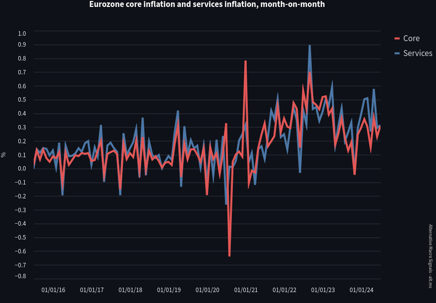
In the Euro area, the stationarity results are more contrasted and somewhat challenging. While headline inflation and core goods HICP are stationary in first difference, the mark is not clearly passed for core inflation and services month-on-month rates, with the bar particularly high for services inflation.
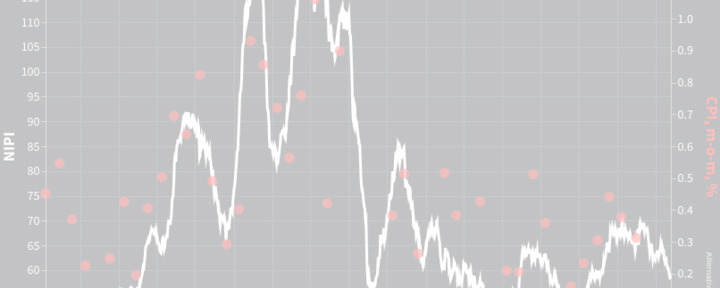
By itself, it is an interesting observation that core inflation data in the euro area exhibits some degree of structural level shift post COVID, as of summer 2024. A casual "visual inspection" can confirm:
Turning to the NIPI data, the indices are most likely to be stationary in level, in theory. Indeed, the NIPIs are constructed as the difference between the volume of positive and negative news, with 50 being neutral. But, again, short sample length and COVID shock, call for proper investigation.
With the same ADF test, we find NIPI the time series pass the stationarity tests in level, as expected, except the euro area Headline HICP which appears "slightly non-stationary" (0.13 p-value in Table 3):
| Region | Name | p-val, level | p-val, diff | Test result |
|---|---|---|---|---|
| US | Headline | 0.045** | - | I(0), level |
| Core | 0.085* | - | I(0), level | |
| Euro area | Headline | 0.126 | 0.000** | I(0), levels + diff |
| Core | 0.063* | - | I(0), level | |
| Note: * denotes 10% significance and ** 5% significance levels. | ||||
As a consequence, we will be running the Granger causality tests on CPI and NIPIs with the following adjustments:
- US supercore in level
- Euro area core inflation and services will be taken in deviation from month-on-month rates to their prior 36-months average (stationarity evidenced in the Table 2 column "diff + trend"). In effect, this is pretty close to allowing a structural level shift, without formally testing it which would be tricky anyway given the sample edge proximity.
- other inflation data to be transformed in month-on-month rates, as expected
- the euro area headline NIPI will be the difference from recent trend (see p-val diff column in Table 3), which can be taken as a "light" I(1) differentiation
- other NIPIs indices will be in level, as expected.
2. VAR Optimal lag choice
Once stationarity dealt with, Granger causality can also be very sensitive to the lag we choose to run the test for.
A vector autoregressive (VAR) model which includes integrated lagged values of both the NIPI and CPI series will be used as a benchmark to determine the optimal lag. We utilize two methods to determine those optimal lags: the Bayesian Information Criteria (BIC) and the Akaike Information Criteria (AIC). They are the most commonly used residuals loss functions and generally provide a reasonable range.
The outcome is an estimated optimal lag of between 2 and 3 months in most cases, which is in line with intuition and very much consistent with what the NIPI has been designed to do - see Table 5 reporting the optimal lags for each CPI-NIPI pair.
| Region | NIPI | Inflation | BIC | AIC |
|---|---|---|---|---|
| US | Headline NIPI | Headline CPI | 2 | 3 |
| Core NIPI | Core CPI | 1 | 3 | |
| Core NIPI | Trimmed Mean | 1 | 8 | |
| Core NIPI | Core Goods | 3 | 4 | |
| Core NIPI | Core Services | 1 | 1 | |
| Euro area | Headline NIPI | Headline HICP | 2 | 2 |
| Core NIPI | Core HICP | 1 | 1 | |
| Core NIPI | Supercore | 3 | 7 | |
| Core NIPI | Core Goods | 1 | 2 | |
| Core NIPI | Services | 1 | 1 |
The outliers here are the "supecore" indices, for which the lags can extend beyond 6 months on one criteria. More on that later. In any case, we will use both AIC and BIC lags in the Granger causality test.
3. Hypothesis Testing
Finally, the Granger causality test itself. The test evaluates the null hypothesis that lagged values of x (e.g. the NIPI) do not help predict y (CPI or HICP inflation).
If the p-value is above a certain threshold, then we cannot reject variable x lags as an explanatory variable for y and x "Granger-causes" y. Said differently, x leads y.
Last technical detail before reviewing the results: we have used both chi-square and F distributions (in short, two ways to compute the stats) and all the below results are identical with the two methods.
We first look at whether the NIPI can Granger-cause CPI (or HICP) inflation. The below table reports the test results, relying on the optimal lags determined in the previous step. When Granger-causality is found for a given NIPI-CPI pair over a given lag, the cell will be green: strong green when the lag is consistent with both AIC and BIC and light green when it is the optimal lag according to just one information criteria.
| Lags | |||||||||
|---|---|---|---|---|---|---|---|---|---|
| CPI / HICP | 1 | 2 | 3 | 4 | 5 | 6 | 7 | 8 | 9 |
| US | |||||||||
| Headline | |||||||||
| Core | |||||||||
| Trimmed mean | |||||||||
| Core goods | |||||||||
| Core services | |||||||||
| Euro area | |||||||||
| Headline | |||||||||
| Core | |||||||||
| Supercore | |||||||||
| Goods | |||||||||
| Services | |||||||||
| Note: a green cell denotes Granger causality from NIPI to inflation, for the given lag consistent with both AIC and BIC. A light green cell denotes Granger causality from NIPI to inflation, for the given lag consistent with either AIC or BIC. Test threshold set at 10%. |
|||||||||
The interpretation is straightforward:
- NIPI leads inflation indices by between 1 and 3 months in most cases
- NIPI leads supercore indices by potentially up to 7-8 months
The bar is not passed for US core goods inflation. But recall we are using overall Core NIPI (there are no core goods or core services NIPI breakdown available) to forecast core goods CPI or services CPI; so there is some information loss in the process.
Overall, it is therefore reasonably well-established that the NIPI has a short-term lead over inflation indices. To the extent that some of those short-term shocks persist, the NIPIs can also lead trend inflation measures (supercore).
Now, what about the reverse relationship? Does the CPI also lead the NIPI?
It would be unsurprising to have a two-ways relationship between the two variables. The NIPI would still be informative owing to its daily frequency, but it may not be "comprehensive enough" to cover every CPI shocks. Table 7 shows the Granger causality results, for the CPI/HICP inflation to predict future NIPI values:
| Lags | |||||||||
|---|---|---|---|---|---|---|---|---|---|
| CPI / HICP | 1 | 2 | 3 | 4 | 5 | 6 | 7 | 8 | 9 |
| US | |||||||||
| Headline | |||||||||
| Core | |||||||||
| Trimmed mean | |||||||||
| Core goods | |||||||||
| Core services | |||||||||
| Euro area | |||||||||
| Headline | |||||||||
| Core | |||||||||
| Supercore | |||||||||
| Goods | |||||||||
| Services | |||||||||
| Note: a green cell denotes Granger causality from inflation to NIPI, for the given lag consistent with both AIC and BIC. A light green cell denotes Granger causality from inflation to NIPI, for the given lag consistent with either AIC or BIC. Test threshold set at 10%. | |||||||||
Interestingly, the CPI-HICP have overall a lower ability to predict future NIPI values than the NIPI has to predict future inflation values, which we find an unexpectedly strong result.
There are a handful of exceptions: most critically US headline inflation in the short term, which possibly imply that some non-core shocks are indeed not fully covered by the NIPI.
There are also a couple of instances (US core goods and EA supercore) where the CPI indices seem to have a long-term predictive power (beyond the first few months): that is very much in line with the intuition that NIPI would in the long term converge towards trend inflation. But those are relatively isolated occurence. In compareason, the NIPI's ability to lead supercore continuously (from very near-term to one semester or more) looks stronger.
Summing-up our main findings:
- the NIPIs lead official inflation rates in the short term
- there is surprisingly little information the NIPIs "miss" in the process
- the NIPIs could be more useful trend inflation gauges than some usual supercore indices
In short, we find the statistical evidence at hand supports using the NIPI as a leading indicator for the inflation momentum.
On a side note, we also learned in the process that Euro area core inflation exhibits some level of structural instability post-COVID.
These results could be further optimized in a number ways: by fully leveraging on the NIPI's daily frequency, adjusting the NIPI's sample window (see an example here), combining with the News Volume Index (exemple here), or including non-linear relationships, for instance.
Large Language Models have a role to play in macroeconomics forecasting, at least the type of LLMs implementation at play here: targeted, supervised learning, with original analyst input to train the Language Model.
We can only stress again that Natural Language Processing opens up whole new ways to compile information. Right now, the limiting factor is our ability to imagine, calibrate and evaluate these new methods.
